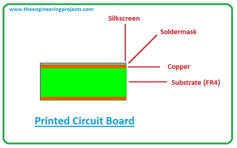
Understanding the Importance of PCB Trace Width

When designing a printed circuit board (PCB), one of the most critical aspects is determining the appropriate trace width for each connection. The trace width directly affects the current-carrying capacity and the overall performance of the PCB. Insufficient trace widths can lead to excessive heat generation, voltage drops, and even circuit failure. On the other hand, overly wide traces can increase manufacturing costs and reduce available space for other components.

Factors Influencing PCB Trace Width

Several factors influence the selection of the appropriate PCB trace width:

1. Current requirements
2. Conductor material
3. Ambient temperature
4. Trace length
5. Acceptable temperature rise

Understanding these factors and their relationships is essential for calculating the optimal trace width for your PCB design.

Calculating PCB Trace Width

To determine the appropriate PCB trace width, you need to consider the current-carrying capacity of the trace. The current-carrying capacity is dependent on several factors, including the conductor material, trace thickness, and ambient temperature.

IPC-2221 Standard

The IPC-2221 standard provides guidelines for determining the current-carrying capacity of PCB traces. This standard takes into account the conductor material, trace thickness, and temperature rise.

According to IPC-2221, the current-carrying capacity of a trace can be calculated using the following formula:

I = k * ΔT^0.44 * A^0.725

Where:
– I = Current-carrying capacity (A)
– k = Constant (dependent on the conductor material and trace thickness)
– ΔT = Temperature rise above ambient (°C)
– A = Cross-sectional area of the trace (mils^2)

The constant k can be determined using the following table:

Conductor Material	Trace Thickness (oz/ft^2)	k
Copper	0.5	0.048
Copper	1	0.024
Copper	2	0.012
Aluminum	0.5	0.054
Aluminum	1	0.027
Aluminum	2	0.013

Calculating Cross-Sectional Area

To use the IPC-2221 formula, you need to calculate the cross-sectional area of the trace. The cross-sectional area is determined by the trace width and thickness.

Trace thickness is typically expressed in ounces per square foot (oz/ft^2). Common trace thicknesses are 0.5 oz/ft^2, 1 oz/ft^2, and 2 oz/ft^2.

To convert the trace thickness from oz/ft^2 to mils, use the following conversion factors:

• 0.5 oz/ft^2 = 0.7 mils
• 1 oz/ft^2 = 1.4 mils
• 2 oz/ft^2 = 2.8 mils

The cross-sectional area can be calculated using the following formula:

A = W * T

Where:
– A = Cross-sectional area (mils^2)
– W = Trace width (mils)
– T = Trace thickness (mils)

Temperature Rise Considerations

The temperature rise (ΔT) used in the IPC-2221 formula is the acceptable increase in temperature above the ambient temperature. The ambient temperature is the temperature of the environment in which the PCB will be operating.

Typical values for acceptable temperature rise range from 10°C to 30°C, depending on the application and the maximum operating temperature of the components on the PCB.

EMSyoCzEBRySapyajbr9zLn2GB+ZrOuLqa4PzHCA8KOg+tXGm3uctfMKVNe67sdd3JuH44jThB6+5qtRRXUlZWR83UqSqSc5bsKKKKZAUUUUAFFFFABRRRQAUUUUAFFFFABRRRQAUUUUAFFFFABRRUsFvc3Mgit4ZJZSCQkSl2IHsKAIq2pG2aDpDlVYLqE7FWGVbGTgj0qt/YfiD/AKBd/wD+A8v+FdJd6PnwppaQ2eptqi3khmga3f8AdZyCSMZ2nqDjv2xyANZbPULTwtBDpunW02vXE9m86QZaLFz5CuvuARnB/DmqFn4e0+/vHtLTVJJiJIYVeKxuHXdIQpZioOFUnBJ//U0Ta/p0egTzaVPHHoVwbiN54plSRmn88CQkcDPHWotN8RS2CPHJaQ3SHUIdTjWV5EVbmJiyswjxkcng8UDCTQrezt2l1LUFtpGmuoLaNYJpfNNv8rElRwM4AyO9XZPBmoR2D3JeQTpYJqDRNbyiMxs2Nom+7uxk49vcZpy+IVubeeC8063uT9oubi0eRiptTcD51XywCR3AJ4wPSobrWo763VbrT4ZL1YBbreCWVH2qflLRoQhIGRkjv7cgE+l2FvqekalDFFH/AGlbXlhMj/8ALRrWZzbOowem54/4eK3LzRNGj1G2vba3T+yYdJupLhG3FGu7TbbSA5LHO54/x+tcvoms3Oh3jXkEUUpeCSCSKcZjdWKuMj2IVh7iph4hvv7IvdIKIy3V7JePOeZR5gBkjHsxCk89vegC/NoSzL9rurq1tbS30qxuZZLe2ON9zLLHHHthHLHaxJx2/GtO+0Pw2smqbpQi2vh/T7q2eGNwryyZBkdVJOeg598+2DH4jlCtBPaRT2b2FtZSW7uyq5tmkeOXcoDZG9u/f8nv4mlmuruaaxt3gudPj05rZSURY4+VIZRnI/z60CNCfQbC+tNBFvcQ29/Lo01yLdYG/wBIaK6nBd5F4BI4Gf7tcfW1H4guY5dNlEEJawsJdPjBLEMjyyTbm9wWP5fjWLQAUUUUAFFFFABRRRQAUUUUAFFFFABRRQATwKAAAngVr2VmIwJZR+8PKg/w/wD16LKz8sCWUfvDyqn+H3+tX65qlS+iPfwOB5bVKm/RBRRVC8vBEGijP7wjDEfw/wD16yjFydkepWrRox55heXvlZjiP7w8E/3f/r1kEkkknJPWgkkkk5J60V1xioo+VxGIlXlzS2CiiirOYKKKKACiiigAooooA6Tan91fyFG1P7q/kKdRXnn29kN2p/dX8hRtT+6v5CnUUBZDdqf3V/IUbU/ur+Qp1FAWQ3an91fyFG1P7q/kKdRQFkN2p/dX8hRtT+6v5CnUUBZDdqf3V/IUbU/ur+Qp1FAWQ3an91fyFG1P7q/kKdRQFkN2p/dX8hRtT+6v5CnUUBZDdqf3V/IUbU/ur+Qp1FAWQ3Yn90flRsT+6Pyp1FAcq7Ddif3V/IUbU/ur+Qp1FAcqG7U/ur+Qo2p/dX8hTqKAshu1P7q/kKNqf3V/IU6igLIbtT+6v5Cjan91fyFOooCyG7U/ur+Qo2p/dX8hTqKAshu1P7q/kKNqf3V/IU6igLIbtT+6v5Cjan91fyFOooCyG7U/ur+Qo2p/dX8hTqKAshu1P7q/kKNqf3V/IU6igLIbtT+6v5Cjan91fyFOooCyG7U/ur+Qo2p/dX8hTqKAsgooqhe3gizFEf3n8RH8P/16qMXJ2RnWrRox55heXnlZjjP7zuf7v/16yCSSSTknrQSSSSck9aK64xUUfK4jESry5pbdEFFFFWcwUUUUAFFFFABRRRQAUUUUAXP7RvPVP++aP7RvPVP++ap0VPJHsdP1qt/Oy5/aN56p/wB80f2jeeqf981Too5I9g+tVv52XP7RvPVP++aP7RvPVP8AvmqdFHJHsH1qt/Oy5/aN56p/3zR/aN56p/3zVOijkj2D61W/nZc/tG89U/75o/tG89U/75qnRRyR7B9arfzsuf2jeeqf980f2jeeqf8AfNU6KOSPYPrVb+dlz+0bz1T/AL5o/tG89U/75qnRRyR7B9arfzsuf2jeeqf980f2jeeqf981Too5I9g+tVv52XP7RvPVP++alt9UkjlR7iJZ4hndGG8ssccfMAf5VnUUuSPYPrVb+dm//bunf9Ag/wDgY/8A8brbmS0h8PWmvfYImWe4MJgW/BeOP5kDH5c5JHTHeuFrZuGb/hHtMGTg30+Rk4OAQKOSPYf1ut/MxbjWraSJkg08QyEjEhuGk24OfulAP8/lR/tG89U/75qnRRyR7C+tVv52XP7RvPVP++aP7RvPVP8AvmqdFPkj2D61W/nZc/tG89U/75o/tG89U/75qnRRyR7B9arfzsuf2jeeqf8AfNH9o3nqn/fNU6KOSPYPrVb+dlz+0bz1T/vmj+0bz1T/AL5qnRRyR7B9arfzsuf2jeeqf980f2jeeqf981Too5I9g+tVv52XP7RvPVP++aP7RvPVP++ap0UckewfWq387Ln9o3nqn/fNH9o3nqn/AHzVOijkj2D61W/nZc/tG89U/wC+aP7RvPVP++ap0UckewfWq387Ln9o3nqn/fNH9o3nqn/fNU6KOSPYPrVb+dlz+0bz1T/vmj+0bz1T/vmqdFHJHsH1qt/Oy099duCC4AIx8oxVXk9aKKaSWxlOpOprN3CiiimZhRRRQAUUUUAFFFFABRRRQAUUUUAaf9lD/nuf++P/ALKj+yh/z3P/AHx/9lWnRXH7SXc+q+oYf+X8X/mZn9lD/nuf++P/ALKj+yh/z3P/AHx/9lWnRR7SXcPqGH/l/F/5mZ/ZQ/57n/vj/wCyo/sof89z/wB8f/ZVp0Ue0l3D6hh/5fxf+Zmf2UP+e5/74/8AsqP7KH/Pc/8AfH/2VadFHtJdw+oYf+X8X/mZn9lD/nuf++P/ALKj+yh/z3P/AHx/9lWnRR7SXcPqGH/l/F/5mZ/ZQ/57n/vj/wCyo/sof89z/wB8f/ZVp0Ue0l3D6hh/5fxf+Zmf2UP+e5/74/8AsqP7KH/Pc/8AfH/2VadFHtJdw+oYf+X8X/mZn9lD/nuf++P/ALKj+yh/z3P/AHx/9lWnRR7SXcPqGH/l/F/5mZ/ZQ/57n/vj/wCyo/sof89z/wB8f/ZVp0Ue0l3D6hh/5fxf+Zmf2UP+e5/74/8Asq1p9NU6Dpyeaci9nYHaOhDZGM/1/wDrMrTm/wCQNp//AF9z/wBaaqS7kywOHVvd/FnM/wBlD/nuf++P/sqP7KH/AD3P/fH/ANlWnRS9pLuV9Qw/8v4v/MzP7KH/AD3P/fH/ANlR/ZQ/57n/AL4/+yrToo9pLuH1DD/y/i/8zM/sof8APc/98f8A2VH9lD/nuf8Avj/7KtOij2ku4fUMP/L+L/zMz+yh/wA9z/3x/wDZUf2UP+e5/wC+P/sq06KPaS7h9Qw/8v4v/MzP7KH/AD3P/fH/ANlR/ZQ/57n/AL4/+yrToo9pLuH1DD/y/i/8zM/sof8APc/98f8A2VH9lD/nuf8Avj/7KtOij2ku4fUMP/L+L/zMz+yh/wA9z/3x/wDZUf2UP+e5/wC+P/sq06KPaS7h9Qw/8v4v/MzP7KH/AD3P/fH/ANlR/ZQ/57n/AL4/+yrToo9pLuH1DD/y/i/8zM/sof8APc/98f8A2VH9lD/nuf8Avj/7KtOij2ku4fUMP/L+L/zMz+yh/wA9z/3x/wDZUf2UP+e5/wC+P/sq06KPaS7h9Qw/8v4v/MzP7KH/AD3P/fH/ANlR/ZQ/57n/AL4/+yrToo9pLuH1DD/y/i/8zLbSyAds2T2BXA/PJrPkjkiYo6kMK6Sq9zbJcJg8OPut6H3q41Xf3jmxGWwcb0VZmDRT5I5ImKOMEfr9KZXSfPtNOzCiiigQUUUUAFFFFABRRRQAUUUUAbv22z/56j8jR9ts/wDnqPyNYVFY+xR639qVeyN37bZ/89R+Ro+22f8Az1H5GsKij2KD+1KvZG79ts/+eo/I0fbbP/nqPyNYVFHsUH9qVeyN37bZ/wDPUfkaPttn/wA9R+RrCoo9ig/tSr2Ru/bbP/nqPyNH22z/AOeo/I1hUUexQf2pV7I3fttn/wA9R+Ro+22f/PUfkawqKPYoP7Uq9kbv22z/AOeo/I0fbbP/AJ6j8jWFRR7FB/alXsjd+22f/PUfkaPttn/z1H5GsKij2KD+1KvZG79ts/8AnqPyNH22z/56j8jWFRR7FB/alXsjd+22f/PUfka1Jry1Giac3mDBvLgDg9ga46rDXc72kNk23yYpWmTj5gzDBGfSj2KJeZ1X0Rq/bbP/AJ6j8jR9ts/+eo/I1hUUexRX9qVeyN37bZ/89R+Ro+22f/PUfkawqKPYoP7Uq9kbv22z/wCeo/I0fbbP/nqPyNYVFHsUH9qVeyN37bZ/89R+Ro+22f8Az1H5GsKij2KD+1KvZG79ts/+eo/I0fbbP/nqPyNYVFHsUH9qVeyN37bZ/wDPUfkaPttn/wA9R+RrCoo9ig/tSr2Ru/bbP/nqPyNH22z/AOeo/I1hUUexQf2pV7I3fttn/wA9R+Ro+22f/PUfkawqKPYoP7Uq9kbv22z/AOeo/I0fbbP/AJ6j8jWFRR7FB/alXsjd+22f/PUfkaPttn/z1H5GsKij2KD+1KvZG79ts/8AnqPyNAvbM4Hmj8jWFRR7FB/alXsjpQQQCOQelLWPZ3pixHKSYz909Sta4IIBHIPSsJRcWezh8RHER5o7kFzbJcIQeHH3W9D71iSRyRMUcYI/X6V0dV7m2juEweHH3W9D71VOpy6PY5cbglWXPD4vzMGinyRvE5Rxgj9fcUyus+bacXZhRRRQIKKKKACiiigAooooAKKKKACiiigAooooAKKKKACiilVWdgqgkk4AFA0r6ISgAnoCfpWrBpqABpzk/wB0cAfUiryxRJ9xFH0ArGVVLY9SjllSavN2Od2t/dP5GkrpSAeoB+tQS2lrL1QA+qcH9OKSrLqjSeVSS9yVzBoq1c2csHzD5o/7wHT61VrZNPVHlVKcqcuWaswooopmYUUUUAFFFFABRRRQAUUUUAFFFFABRU9vay3B+XhR1Y9PwrVisraID5d7dy/P6dKzlUUTtw+CqV9Vou5ibWP8J/I0EEdQR9RXSAKOAAB7DFIyRv8AeRW/3gD/ADrP23kd7ynTSf4HN0Vrz6dE+WiOxuuDyprKkjkiYo4IYVrGalseZXwtSg/fWncbRRRVnMFFFFABRRRQAUUUUAFXrO8MREch/dnoT/D/APWqjRUyipKzNaNaVGXPA6UEEAjkHpS1j2d4YiI5D+77E/w//WrXBBAI5B6VySi4s+qw+IjiI80d+xBc20dwmDw45Vh1z6GsSSN4nKOMEfr7iujqGa3hn2+YudpyCOD9MiqhU5dGc2MwSr+9DSX5nP8ANLtf+635GuhSCCMAJGo98ZP5nmn4HTFX7byOSOUu3vS/A5qiugktraUHdGufUDB/MVmXNg8WXjJZO47qKuNVM5a+X1KS5lqilRRRWp5wUUUUAFFaX9lt/wA9R/3zR/Zbf89R/wB81n7SPc7fqGI/l/IzaK0v7Lb/AJ6j/vmj+y2/56j/AL5o9pHuH1DEfy/kZtFaX9lt/wA9R/3zR/Zbf89R/wB80e0j3D6hiP5fyM2itL+y2/56j/vmj+y2/wCeo/75o9pHuH1DEfy/kZtbVlaiFA7D944/75B7c1FHpuyRHaQMFYNjHXBzWjWVSpfRHpYDBypyc6q16BRRRWB7IUUUUAIQGBBGQRgg+lYd5bG3k4/1b8ofT2rdqrex+ZbvxynzD8K0py5WcOOoKtSb6ow6KKK7D5UKKKKACiiigAooooAKKKKACpreBp5Ag6dWPoKhrY02ILC0neRv/HV4/wAaicuVXOvB0fbVVF7dS4iJGqogwqjAFOooriPrEklZBRRRQMKrXdstxGf+eijKH+lWaKadndEVIRqRcZbM5ogqSCMEHB/Ckq5qEXlz7gOJBu/HvVOu6Lurnx9am6U3B9AooopmQUUUUAFFFFABRRRQAVes7zysRyk+WeFJ/hqjT4kMkkaf3mUH6E1MkmtTahUnTmnDc6IEEAjkHpS0igKFUdAAB+FLXCfZLzCiiigAooooAx7+1ETeag+Rz8wA4U1RroZ4xLFIh7g4+tc8QQSD1HBrrpSutT5nMKCpVOaOzCiiitTzTpqKrfbbP/nqPyP+FH22z/56j8j/AIVw8r7H2X1il/MvvLNFVvttn/z1H5H/AAo+22f/AD1H5H/CjlfYPrFL+ZfeWaKrfbbP/nqPyP8AhR9ts/8AnqPyP+FHK+wfWKX8y+8s0VW+22f/AD1H5H/Cj7bZ/wDPUfkf8KOV9g+sUv5l95ZoqBbu1dlVZAWY4AwanpNNblxnGesXcKKKKRZo6n/q9D/7BUX/AKPmrOrR1P8A1eh/9gqL/wBHzVnU2RD4QpkgBjkB6bW/lW1/ZNobFb5dSiaN5mtkXybne1wsayeXgRn1Hfv1rOuNO1hY3QafemRoi6oLebcVzt3Y25xmmk7kSqx5Wzk6KtQ6fqdxJPDBZXUksBInjjhkZ4iMjDqBkHg/lQmnapJDLcR2V20ERYSyrBIY0KZ3BmAxx39K7j40q0Vp6XpL6kuoTGeOC2sIRcXUsiSvtQ5AwsKs3XjpUf8AZV7NPNFp0c2oxpIIxPY29w8bE9OGQMM+4FAFCircOmavcG4WCwvJWtmK3Ajt5WMTA42uAOD7UkGnapcxyzW9jdzQw7vNkhgldE2qWO5lBAwASfp7UAVaK0G0u8eSKOygvLlntoLhglrMGHmccLjJXPAPQ1Gml6xJcS2ken3rXURAlgW3lMseTgb025H4igCnRUs9vc2sskFzDJDNGcSRzKyOp9GVuaioAK37QAW8OP7v9awK27CQPbIO6Eof51jW2PWyuSVVryLdFFFcp9EFFFFABRRRQBmaoBiA9/mFZlaGpvmSNB/CuT9TWfXZT+FHymOadeVgooorQ4gooooAKKKKACiiigAq1YAG6iz/ALR/JSaq1NbP5c8LHpvAJ9jwamWzNqDUasW+6OgooorhPsgooooAKKKKACucm4mmH/TR/wD0I10LsFR2PAAJrnGO5mb+8xP5nNdFHqeJmzVor1EoooroPCCiiigAooooAKKKKACiiigBVZkZWU4ZSGB9xzW/bzLPGrjGejD0PpXP1Nb3Elu+5eQfvKehFZ1IcyO/BYr2E/e2Z0FFQw3MM4BRhu7qfvCpq5Grbn08ZRmuaLujR1P/AFeh/wDYKi/9HzVnVs63ZXlpDoDTxbFk01EQ70YMyyPIQNhPZlP41ikgDJIA9+KHuTTknG6Nu1vLOPTNOt3lAmi1w3cibW+WDZCu/IGP4T3qNtW0a71bXJb6/AxOslk1x9qFvIu9wQywROeBt2grjk+lcvdagozHAcnoX7D2FZfXmuinF7s8PHYiGsKbv3O5v9S0XUDrlrb6tDZGXUbW7ju2hu9l1CtrDCyZiiMg2lWIyo6+/wAr4Nc0uLT9M+zXmnLdWMN9BIL2K+3Ss88jiVBFCyEMGyckHqDXB0VueQbOgXD2txNNHrEWmSBFUGeO4kinRjh0ZYI3PT1A+tdVK+jXmma5/Z9/badaPfWEXniG5ige4SOISsqxqzhWIJXKj3xnjzyniWYRtEHYRM25kBIUnjkj8BQB6Fb6z4Wl1efUX1BIzDqds6vdR3g+0wQ7d06JBGw3NgEbsVj3V3pV7YCKHVorJrW81OVoXiugLxJmLxlPKjZfRRux19ueSooEddJrOnrZagkF3ieXw1pVhFsWUMbiK4haRAdvGAG5z/8AX3rO5069t7+5WQywiPQoJHEd4D9qhWd8FrWN5+O/y4OMZyQK8zqaC6vLYsbeeWIsMN5TsufrigZf8RJeR6xqIu3gecurM1sxMZBRduMgN0x1APtzWVSszuzO5LMxJYnkkmkAJIAGSeBQIACSABkngVt2Nu0EZLH5pMEjsMdKjs7IRgSyDMh6D+7V+uapUvoj6HAYN0/3s9+gUUUgKnoQfoc1geuLRRRQAUySRIkZ3OAoz9T6CmyzwwqS7Aeg7n8Kxrq6e4b0QH5V/qa0hByOHFYuNCNl8RFLI0sjyN1Y5+lMoorsPlm3J3YUUUUCCiiigAooooAKKKKACiiigDcsrgTRAE/OnDDuferVc5FLJC4dDgj16Eehrat7yGcAZCv3U/0NctSnZ3R9JgsZGpFQm/e/Ms0UUVieoFFFUrm/jiBSIh5OnH3V+ppqLlojKrVhSjzTYzUbgKnkqfmbl8dh6GsmlZmdmZjksck0ldsI8qsfK4mu69RzYUUUVRzBRRRQAUUUUAFFFFABRRRQAUUUUAS28kMUyPNE0sa7t0ayGItkED5wD069K1U1fTkxjTZiB2a+Yj/0VmsWik0nuaQqTh8LsdJc+JobuO2jnsJWW2iEMH+mt+7jB3YGY/8AP4cZt1fWNxGypZzxy/wu14ZFHrlPLH8x/Q5tFHKkOVapJWcnYKKKKZkFXbGyF4uosZCn2Symuxhd28x87eoqlWxon3PEH/YHvP5CgDHooooAKKKKACiigAkgAZJ4FAAASQAMk8CtezsxGBLKAXP3R/d+tFnZiMCWQZcj5R/dq/XNUqX0R7+BwPLapUWvRBRRWffXmweVEfmI+dh/CPSsoxcnZHp1q0aMOeQl7ehcxQn5ujsO3sKzUmmjOUdgfrTKK64wUVY+WrYmdafO3bt5FsahdgYyp9yvNI1/dt/GB/ujFVaKfJHsL6zWatzP7xWZmOWJJ9Sc0lFFUc+4UUUUAFFFFABRRRQAUUUUAFFFFABRRRQAUcjpRRQBOl3dR8CQkejcipf7Ru/VP++f/r1ToqeWL6G8cRVirKTJpLm5l+9I2PQcD9KhooppJbGUpym7ydwooopkhRRRQBf/ALMn/vp+tH9mT/30/WteiuT2sj6f+zaHb8TI/syf++n60f2ZP/fT9a16KPayD+zaHb8TI/syf++n60f2ZP8A30/Wteij2sg/s2h2/EyP7Mn/AL6frR/Zk/8AfT9a16KPayD+zaHb8TI/syf++n60f2ZP/fT9a16KPayD+zaHb8TMg0sGWMXExSHP7xol3OBj+EMQP1q6NI0XjN5e9s4t4/8AZzj95/vfp6czUUe1kH9m0O34ktx4YsrSGwuLi4vVivYzLC32dBuVdm7q/ufzH40JtJ04RMYLu4aYYwssCKh4GcsHJ9e3+J6XWLm5lsPDkckrun2NpMMc4YOUyPwrEpurIinl9FxvJd+vmZH9mT/30/Wj+zJ/76frWvRS9rIv+zaHb8TI/syf++n61raNp86LrgLph9IvFyM53EDFLWlpX3dY/wCwZdfyFCqyJll1BK6X4nLf2ZP/AH0/Wj+zJ/76frWvRR7WRX9m0O34mR/Zk/8AfT9aP7Mn/vp+ta9FHtZB/ZtDt+Jkf2ZP/fT9as2tiISXkIZ/4cdB71eopOpJqxpTwNGnLmS1CiiqF5eiMGKIgyH7x/u//XqYxcnZHRWrRox55he3ojBiiOZCPmYfw/8A16yCSSSTknrQSSSSck9aK64xUUfK4jESry5pbBRRRVnMFFFFABRRRQAUUUUAFFFFABRRRQAUUUUAFFFFABRRRQAUUUUAFFFFABRRRQAUUUUAFFFFAHQ+fb/89U/MUefb/wDPRPzFc9RWHsV3PZ/taf8AKjofPt/+eifmKPPt/wDnon5iueoo9iu4f2tP+VHQ+fb/APPRPzFHn2//AD0T8xXPUUexXcP7Wn/KjofPt/8Anon5ijz7f/non5iueoo9iu4f2tP+VHQ+fb/89E/MUefb/wDPRPzFc9RR7Fdw/taf8qOh8+3/AOeifmKPPt/+eifmK56ij2K7h/a0/wCVHcarPbiy8N/vU5sHI+YdPNNZHn2//PRPzFRa1/yD/Cn/AGDX/wDRzVh0Oin1Jjmk4q3KjofPt/8Anon5ijz7f/non5iueoo9iu5X9rT/AJUddFY3s0aSxRFo3GUYMmCPXk1u6FbwWw1YajZSv5tjLHBslVcseqcMOvGDXmlFNUkjOeZzmuXl/M7H+zdS/wCfc/8AfSf/ABVU5iLeV4ZiqSpt3KSMjcAw6VzVFL2K7l/2rP8AlR0Pn2//AD0T8xR59v8A89E/MVz1FHsV3H/a0/5UdD59v/z0T8xQbi3AJMqYHvXPUUexXcP7Wn/KjVutQQKUgOWPBfsB7VlEkkknJPUmiitYxUVoedXxE68uaYUUUVRzhRRRQAUUUUAFFFFABRRRQAUUUUAFFFFABRRRQAUUUUAFFFFABRRRQAUUUUAFFFFABRRRQAUUUUAGD6GjB9DXSbE/ur+Qo2R/3F/IVz+28j2/7Jf8/wCBzeD6GjB9DXSbI/7i/kKNkf8AcX8hR7byD+yX/P8Agc3g+howfQ10myP+4v5CjZH/AHF/IUe28g/sl/z/AIHN4PoaMH0NdJsj/uL+Qo2R/wBxfyFHtvIP7Jf8/wCBzeD6GjB9DXSbI/7i/kKNkf8AcX8hR7byD+yX/P8Agc3g+howfQ10myP+4v5CjZH/AHF/IUe28g/sl/z/AIFfWgf7P8K/9g5//RzVh4Poa7C7uY7mDTYREF+x25hJODuy2cj/AD/KqeyP+4v5Cn7byEsqb3l+BzeD6GjB9DXSbI/7i/kKNkf9xfyFL23kP+yX/P8AgYKWl46q6QSsrdCqkg84p32G/wD+fab/AL4PriukS7vo1VEurhEUAKqSyKqgdgAcVueHrqGSfUBqVzfOq6fcyRBJZGAKIWZuucgfd9/1arXexE8rcIuXN+B5/wDYb/j/AEab/vg1C8ckbFHRlYYyrAgjIz0Ndab7UcnF7d4zx+/l6fnVZyZXaSQl3bBZ3+ZmI9SeaXtvIv8Asl/z/gczg+howfQ10myP+4v5CjZH/cX8hR7byD+yX/P+BzeD6GjB9DXSbI/7i/kKNkf9xfyFHtvIP7Jf8/4HN0Vs3VlHKpaNQsg544DexFY7KyMVYYYHBBrWM1I87EYWeHdpbdxKKKKs5QooooAKKKKACiiigAooooAKKKKACiiigAooooAKKKKACiiigAooooAKKKKACiiigAooooAKKKKAOmorF/tG79V/75FH9o3fqv8A3zXJ7KR9L/adDz+42qKxf7Ru/Vf++aP7Ru/Vf++aPZSD+06Hn9xtUVi/2jd+q/8AfNH9o3fqv/fNHspB/adDz+42qKxf7Ru/Vf8Avmj+0bv1X/vmj2Ug/tOh5/cbVFYv9o3fqv8A3zR/aN36r/3zR7KQf2nQ8/uNqisX+0bv1X/vmj+0bv1X/vmj2Ug/tOh5/cbVFYv9o3fqv/fNH9o3fqv/AHzR7KQf2nQ8/uNqisX+0bv1X/vmj+0bv1X/AL5o9lIP7Toef3G1Wlo/+vvv+wZqP/olq5P+0bv1X/vmtjQLy5km1bcV/d6LqUi4UfeEYX+tNUpEzzKi4tK46isX+0bv1T/vmj+0bv1X/vml7KRX9p0PP7jaorF/tG79V/75o/tG79V/75o9lIP7Toef3G1RWL/aN36r/wB81ZtdQLtsmwCT8rDgfQ0nSklcunmFGclFaGjVS7tFnG5cCUDg+vsat0VCbTujsqU41Y8s1oc0ysjFWGGBwQaStu7tFnBZcCUDg+vsaxWVkZlYEMDgg12QmpI+WxWFlh5We3RiUUUVZyBRRRQAUUUUAFFFFABRRRQAUUUUAFFFFABRRRQAUUUUAFFFFABRRRQAUUUUAFFFFABRRRQAUUUUAFFFFABRRRQAUUUUAFFFFABRRUkce/HOOQOnrxQOMXJ2RHRVlrYAE7zx7f8A16rkYOKSaZc6cofEJRRRTMwrc8Of67Wv+wFqf/oC1h1ueHP9drX/AGAtT/8AQFoAw6KKKACiiigAooooA07K9+7DMfZGP8jWnXM1rafcSSBon52AENnnHoa56lO3vI93AYxyapVPkaFVLu0WcblwJAOD6+xq3RWCbTuj16lONWLjJaHNMrIzKwIZTgg9QaStm+t43jaXo6jqO/saxh1FdkJcyufK4rDvDz5X8goqwlsGXO/H4UySLYSN2fw9s1XMjJ0ppczRFRRRTMgooooAKKKKACiiigAooooAKKKKACiiigAooooAKKcibu+KsG1ABO88Anp/9ek2kaRpSmrpFWinMu04znr+lNpkNWCiiigQUUUUAf/Z” alt=”” class=”wp-image-136″ >

Putting It All Together

Now that we have covered the factors influencing PCB trace width and the IPC-2221 standard for calculating current-carrying capacity, let’s walk through an example calculation.

Example Calculation

Suppose we have the following design requirements:
– Conductor material: Copper
– Trace thickness: 1 oz/ft^2
– Current requirement: 2A
– Ambient temperature: 25°C
– Acceptable temperature rise: 20°C

Step 1: Determine the constant k based on the conductor material and trace thickness.
From the table above, for copper with a trace thickness of 1 oz/ft^2, k = 0.024.

Step 2: Convert the trace thickness from oz/ft^2 to mils.
1 oz/ft^2 = 1.4 mils

Step 3: Calculate the cross-sectional area (A) required to carry the desired current.
Using the IPC-2221 formula:
2 = 0.024 * 20^0.44 * A^0.725

Solving for A:
A = (2 / (0.024 * 20^0.44))^(1/0.725) = 205.6 mils^2

Step 4: Calculate the required trace width (W).
Using the cross-sectional area formula:
205.6 = W * 1.4

Solving for W:
W = 205.6 / 1.4 = 147 mils

Therefore, to carry a current of 2A with a copper trace of 1 oz/ft^2 thickness and an acceptable temperature rise of 20°C above an ambient temperature of 25°C, the trace width should be at least 147 mils.

Additional Considerations

When designing PCB traces, there are a few additional factors to consider:

Voltage Drop

Voltage drop occurs when current flows through a conductor with resistance. The voltage drop can be calculated using Ohm’s law:

V = I * R

Where:
– V = Voltage drop (V)
– I = Current (A)
– R = Resistance (Ω)

The resistance of a trace can be calculated using the following formula:

R = ρ * L / A

Where:
– R = Resistance (Ω)
– ρ = Resistivity of the conductor material (Ω * mil)
– L = Trace length (mils)
– A = Cross-sectional area (mils^2)

To minimize voltage drop, ensure that the trace width is sufficient to maintain an acceptable resistance for the given current and trace length.

High-Frequency Considerations

For high-frequency signals, it is essential to consider the skin effect and the characteristic impedance of the traces.

The skin effect causes high-frequency currents to flow primarily on the surface of a conductor, effectively reducing the cross-sectional area and increasing the resistance. To mitigate the skin effect, consider using wider traces or multiple parallel traces for high-frequency signals.

Characteristic impedance is the ratio of the voltage to the current in a transmission line. Matching the characteristic impedance of the traces to the source and load impedances is crucial for minimizing signal reflections and ensuring Signal Integrity. The characteristic impedance can be controlled by adjusting the trace width, thickness, and the distance between the trace and the reference plane (e.g., ground or power plane).

Manufacturing Constraints

When determining PCB trace widths, it is essential to consider the manufacturing capabilities of your PCB fabricator. Minimum trace width and spacing requirements may vary depending on the fabricator and the chosen manufacturing process.

Consult with your PCB fabricator to ensure that your designed trace widths are compatible with their manufacturing capabilities and design rules.

Frequently Asked Questions (FAQ)

1. What happens if the PCB trace width is too narrow for the current requirements?
   If the PCB trace width is too narrow for the current requirements, it can lead to several issues:
2. Excessive heat generation due to increased resistance
3. Voltage drops across the trace
4. Increased risk of trace damage or failure due to overcurrent

5. Reduced performance and reliability of the circuit
   To avoid these issues, ensure that the trace width is sufficient to handle the expected current based on the IPC-2221 guidelines or other relevant standards.

6. Can I use different trace widths for different sections of the same net?
   Yes, you can use different trace widths for different sections of the same net. This is often done to optimize space utilization and accommodate varying current requirements along the net.
   For example, you may use a wider trace width for sections of the net that carry higher currents, such as near power sources or high-current components, and narrower trace widths for sections with lower current requirements.
   When changing trace widths along a net, ensure that the transitions are gradual to minimize impedance discontinuities and signal reflections.

7. How does the ambient temperature affect the required trace width?
   The ambient temperature affects the required trace width by influencing the acceptable temperature rise. As the ambient temperature increases, the acceptable temperature rise decreases, requiring wider traces to maintain the same current-carrying capacity.
   For example, if the ambient temperature is 50°C and the maximum operating temperature of the components is 80°C, the acceptable temperature rise is only 30°C. In contrast, if the ambient temperature is 25°C, the acceptable temperature rise can be higher, allowing for narrower traces.
   When designing PCBs for high-temperature environments, it is crucial to consider the ambient temperature and adjust the trace widths accordingly.

8. What are the consequences of using overly wide traces?
   While using wider traces than necessary ensures sufficient current-carrying capacity, there are some drawbacks to using overly wide traces:

9. Increased manufacturing costs due to the increased use of copper
10. Reduced available space for other components and traces
11. Potential impact on signal integrity, especially for high-frequency signals

12. Increased capacitance between traces, which may affect signal timing and propagation
    To optimize your PCB design, aim to use trace widths that are sufficient for the current requirements while minimizing excess copper usage.

13. Can I use online calculators or software to determine PCB trace widths?
    Yes, there are many online calculators and PCB design software tools that can help you determine the appropriate PCB trace widths based on your design requirements.
    These tools typically take into account factors such as the conductor material, trace thickness, current requirements, and ambient temperature, and provide recommendations based on industry standards like IPC-2221.
    However, it is essential to understand the underlying principles and calculations to ensure that the results provided by these tools are appropriate for your specific design. Always verify the results and consult with experienced PCB designers or engineers when in doubt.

Conclusion

Determining the appropriate PCB trace width is a critical aspect of PCB design, as it directly affects the current-carrying capacity, performance, and reliability of the circuit. By understanding the factors that influence trace width, such as current requirements, conductor material, ambient temperature, and acceptable temperature rise, you can calculate the optimal trace width using industry standards like IPC-2221.

Remember to consider additional factors such as voltage drop, high-frequency considerations, and manufacturing constraints when designing your PCB traces. By following these guidelines and working closely with your PCB fabricator, you can ensure that your PCB design is optimized for performance, reliability, and manufacturability.